So far we have taken small bits of OpenCV goodness and explored them independently. Today we are going to see how we can combine a few things together and build ourselves a small app that helps us convert a coloured image into its Hue, Saturation and Value equivalent, and then adjust the HSV range to isolate one or more colours in the image.

To do this we'll need to

• Load an image from disk (later we'll do this on a video frame)
• Show it in a window
• Add multiple trackbars to the window so we can adjust the HSV values
• Respond to trackbar changes and adjust HSV values of the image on-the-fly

We are going to use the following image to determine the HSV values that best identify each ball separately.

Building a small GUI with trackbars in OpenCV

Python OpenCV seems to support a subset of all things OpenCV can do when you work with a toolkit like Qt. So unfortunately we can't create a fully functional media-player in Python (or I haven't found the correct documentation to do this).

However, it does support trackbars/slider component, which is all we need to make our calibration tool.

Colour thresholding using HSV values in OpenCV works within a range of 'lower HSV values' and 'upper HSV values'. This means we need six track bars to tweak each value independently. We'll store the values in the following variables: uh, us, uv, lh, ls and lv. I have set them to an initial value that should track some blue in an image.

import numpy as np
import cv2 as cv
import time

img = cv.imread('./SampleImages/All.jpg',cv.IMREAD_COLOR)
img = cv.medianBlur(img,5)

# Convert BGR to HSV
hsv = cv.cvtColor(img, cv.COLOR_BGR2HSV)

uh = 130
us = 255
uv = 255
lh = 110
ls = 50
lv = 50
lower_hsv = np.array([lh,ls,lv])
upper_hsv = np.array([uh,us,uv])

We have the target ranges now, lets apply the thresholding and get the masked image. Thanks to OpenCV, it's a single line of code.

# Threshold the HSV image to get only blue colors
mask = cv.inRange(hsv, lower_hsv, upper_hsv)

Since we are going need a reference to the window to which the trackbars need to be added, we'll create a namedWindow

window_name = "HSV Calibrator"
cv.namedWindow(window_name)

To create simple trackbars that span the entire length of the parent window we initialise a trackbar component with a name, min and max values, the parent window's name and a delegate function that is called whenever the particular tracker is using. While this is a good way to track changed values, we will for now use the main while loop to retrieve values from the trackbars. But before that we setup the trackbars and assign initial values as defined above:

def nothing(x):
    print("Trackbar value: " + str(x))
    pass

# create trackbars for Upper HSV
cv.createTrackbar('UpperH',window_name,0,255,nothing)
cv.setTrackbarPos('UpperH',window_name, uh)

cv.createTrackbar('UpperS',window_name,0,255,nothing)
cv.setTrackbarPos('UpperS',window_name, us)

cv.createTrackbar('UpperV',window_name,0,255,nothing)
cv.setTrackbarPos('UpperV',window_name, uv)

# create trackbars for Lower HSV
cv.createTrackbar('LowerH',window_name,0,255,nothing)
cv.setTrackbarPos('LowerH',window_name, lh)

cv.createTrackbar('LowerS',window_name,0,255,nothing)
cv.setTrackbarPos('LowerS',window_name, ls)

cv.createTrackbar('LowerV',window_name,0,255,nothing)
cv.setTrackbarPos('LowerV',window_name, lv)

font = cv.FONT_HERSHEY_SIMPLEX

Next we start our main loop.

We get a masked version of the HSV image with latest values in lower_hsv and upper_hsv. These values are updated as the trackbar values change.

To help note down values that work the best I am printing the lower and upper hsv values on the top left corner of the screen.

We show the masked image in our named window using cv.imshow(window_name,mask)

We have a handler to close the application if user presses the Esc key.

Finally we simply grab the current value of each tracker and update the upper_hsv and lower_hsv

To keep CPU usage optimal we sleep for 100 milliseconds (without this you could run the CPU at 100%, on my VM I went from 80% to ~5% when I added the time.sleep(.1)

while(1):
    # Threshold the HSV image to get only blue colors
    mask = cv.inRange(hsv, lower_hsv, upper_hsv)
    cv.putText(mask,'Lower HSV: [' + str(lh) +',' + str(ls) + ',' + str(lv) + ']', (10,30), font, 0.5, (200,255,155), 1, cv.LINE_AA)
    cv.putText(mask,'Upper HSV: [' + str(uh) +',' + str(us) + ',' + str(uv) + ']', (10,60), font, 0.5, (200,255,155), 1, cv.LINE_AA)

    cv.imshow(window_name,mask)

    k = cv.waitKey(1) & 0xFF
    if k == 27:
        break
    # get current positions of Upper HSV trackbars
    uh = cv.getTrackbarPos('UpperH',window_name)
    us = cv.getTrackbarPos('UpperS',window_name)
    uv = cv.getTrackbarPos('UpperV',window_name)
    upper_blue = np.array([uh,us,uv])
    # get current positions of Lower HSCV trackbars
    lh = cv.getTrackbarPos('LowerH',window_name)
    ls = cv.getTrackbarPos('LowerS',window_name)
    lv = cv.getTrackbarPos('LowerV',window_name)
    upper_hsv = np.array([uh,us,uv])
    lower_hsv = np.array([lh,ls,lv])

    time.sleep(.1)

cv.destroyAllWindows()

Calibrating for various colours

Now that we have the application going we let it run and it should come up with something like this by default.

The main white area is the blue ball, the white speckles around it is noise. We should be able to move the sliders around to keep most of the ball white while making the rest of the background completely black.

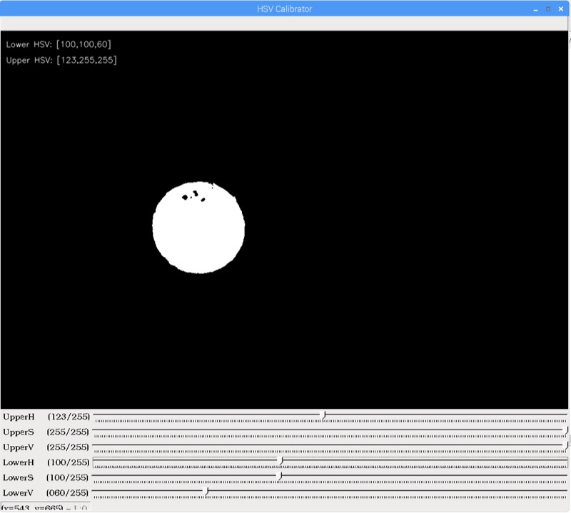
After careful manipulation we get the following image

The HSV values for this image is:
Blue Lower HSV : [100,100, 60]
Blue Upper HSV : [123,255,255]

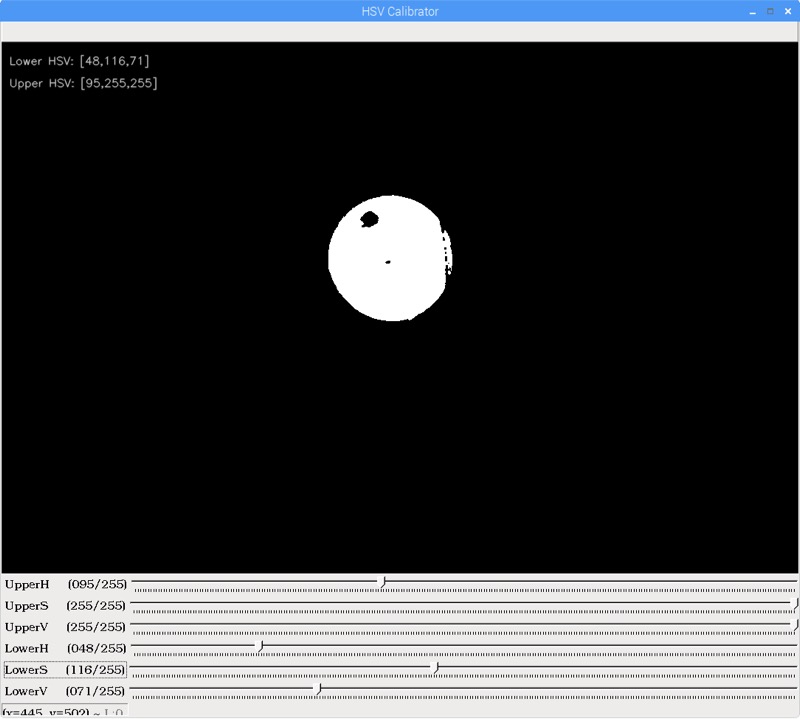
Now lets try and get the next ball Green's position

We have to play around a little with the trackbars till see the green ball only on screen and we note down the values as Green Lower HSV: [ 48,116, 71]
Green Upper HSV: [ 92,255,255]

The next colour we try to isolate is Yellow position The yellow one comes out optimised at Yellow Lower HSV: [ 18, 74,128] Yellow Upper HSV: [ 47,240,255]

Finally we have the red left and after quite a bit of experimenting we end up with the following isolated mask for the red ball. You will see the red ball comes out the worst of the lot. After the intial confusion, if you go back and look at the coloured image again, you'll see why. The parts that come out black towards the bottom of the ball actually look brown if you look closely. Human eyes and brain wire things up to form the coherent ball shape in our head. Unfortunately a computer can do that straightaway because it works binary, No/Yess or 0/1 or off/on. To grey things out you've to get it work a little harder.

Conclusion

To wrap up, we saw how we could up with HSV threshold ranges that could help us identify colours in an image.

Next challenge is to find position of objects based on the colour thresholds we just identified. So we'll grab a video feed and try to analyse position of ball at runtime based on above determined HSV values for each colour.